Tracking sampled hyperparameters
In some cases we are not only interested in the best hyperparameter. Instead we also want to visualize and analyze which hyperparamter ranges result in a high objective value.
For such cases we can use the pyhopper.callbacks.History() callback, which takes care of recording and organizing the evaluated hyperparameters.
import numpy as np
import matplotlib.pyplot as plt
import pyhopper
def gauss(x, y, mux, muy, sx, sy):
return np.exp(-1 / sx * np.square(x - mux)) * np.exp(-1 / sy * np.square(y - muy))
def objective(x, y):
v = gauss(config["x"], config["y"], 2, 5, 10, 5)
v -= 1.2 * gauss(config["x"], config["y"], 3, 4, 50, 5)
v += 0.3 * gauss(config["x"], config["y"], -3, -7, 80, 20)
v += gauss(config["x"], config["y"], 5, 3, 50, 100)
return v
search = pyhopper.Search(
{
"x": pyhopper.float(-10, 10),
"y": pyhopper.float(-10, 10),
},
)
history = pyhopper.callbacks.History()
search.run(objective, direction="max", seeding_steps=10, max_steps=50, callbacks=history)
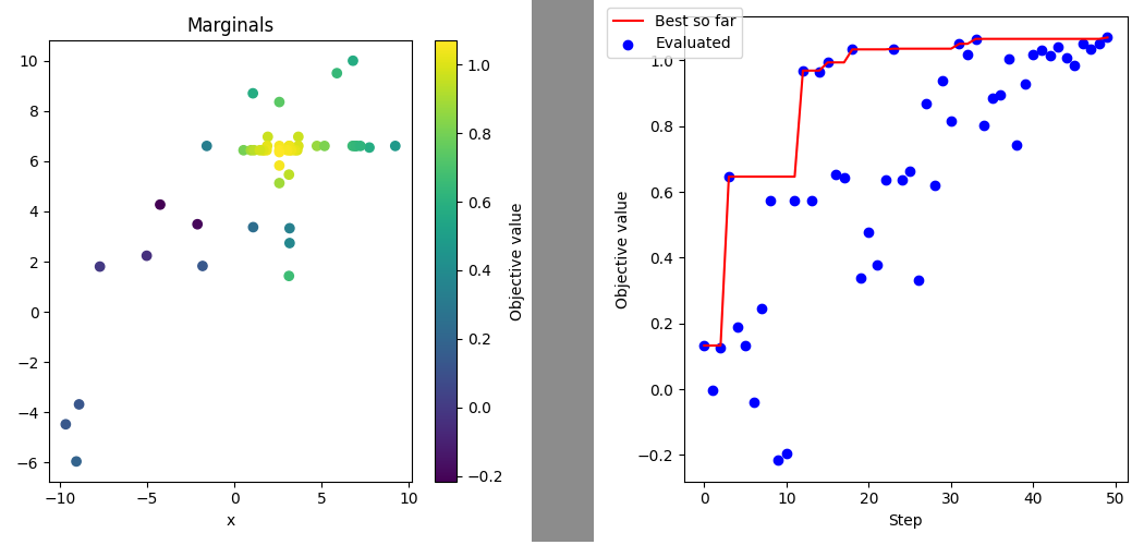
# Let's plot the sampled parameters as the 2D objective surface
fig, ax = plt.subplots(figsize=(5, 5))
b = ax.scatter(
x=history.get_marginal("x"),
y=history.get_marginal("y"),
c=history.fs,
)
ax.set_xlabel("y")
ax.set_xlabel("x")
ax.set_title("Marginals")
fig.colorbar(b, ax=ax, label="Objective value")
fig.tight_layout()
fig.savefig("marginal.png")
plt.close(fig)
# Let's plot evaluated objective values over the optimization process
fig, ax = plt.subplots(figsize=(5, 5))
ax.plot(history.steps, history.best_fs, color="red", label="Best so far")
ax.scatter(x=history.steps, y=history.fs, color="blue", label="Evaluated")
ax.set_xlabel("Step")
ax.set_ylabel("Objective value")
fig.legend(loc="upper left")
fig.tight_layout()
fig.savefig("search.png")
plt.close(fig)
will generate the figures marginal.png and search.png