Search history#
In some cases we are not only interested in the best hyperparameter but the entire distribution of hyperparameters and
corresponding objective values.
Pyhopper keeps track of all evaluated candidates in the pyhopper.Search.history property.
import numpy as np
import matplotlib.pyplot as plt
import pyhopper
def gauss(x, y, mux, muy, sx, sy):
return np.exp(-1 / sx * np.square(x - mux)) * np.exp(-1 / sy * np.square(y - muy))
def objective(x, y):
v = gauss(config["x"], config["y"], 2, 5, 10, 5)
v -= 1.2 * gauss(config["x"], config["y"], 3, 4, 50, 5)
v += 0.3 * gauss(config["x"], config["y"], -3, -7, 80, 20)
v += gauss(config["x"], config["y"], 5, 3, 50, 100)
return v
search = pyhopper.Search(
{
"x": pyhopper.float(-10, 10),
"y": pyhopper.float(-10, 10),
},
)
search.run(objective, direction="max", seeding_steps=10, steps=50)
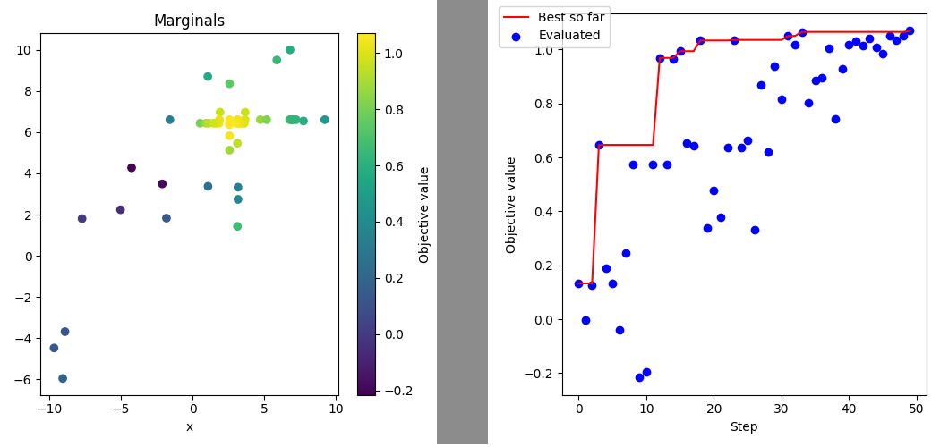
# Let's plot the sampled parameters as the 2D objective surface
fig, ax = plt.subplots(figsize=(5, 5))
b = ax.scatter(
x=search.history["x"],
y=search.history["y"],
c=search.history.fs,
)
ax.set_ylabel("y")
ax.set_xlabel("x")
ax.set_title("Marginals")
fig.colorbar(b, ax=ax, label="Objective value")
fig.tight_layout()
fig.savefig("marginal.png")
plt.close(fig)
# Let's plot evaluated objective values over the optimization process
fig, ax = plt.subplots(figsize=(5, 5))
ax.plot(search.history.steps, search.history.best_fs, color="red", label="Best so far")
ax.scatter(x=search.history.steps, y=search.history.fs, color="blue", label="Evaluated")
ax.set_xlabel("Step")
ax.set_ylabel("Objective value")
fig.legend(loc="upper left")
fig.tight_layout()
fig.savefig("search.png")
plt.close(fig)
will generate the figures marginal.png and search.png