Quickstart#
This is the quickstart guide of PyHopper
The Search class#
The central component of PyHopper is the pyhopper.Search() class whose constructor defines the search space and run method performs the hyperparameter search.
For example
import pyhopper

def dummy_objective(param :dict) -> float:
    print(param)
    return 0

search = pyhopper.Search(
    {
        "my_const": "cifar10",
        "my_int": pyhopper.int(100,500),
        "my_float": pyhopper.float(0,0.4),
        "my_choice": pyhopper.choice(["adam","rmsprop","sgd"]),
    }
)
search.run(dummy_objective,"maximize",steps=5,quiet=True)
outputs
> {'my_const': 'cifar10', 'my_int': 364, 'my_float': 0.3404501564, 'my_choice': 'sgd'}
> {'my_const': 'cifar10', 'my_int': 408, 'my_float': 0.1056544366, 'my_choice': 'adam'}
> {'my_const': 'cifar10', 'my_int': 206, 'my_float': 0.2091606387, 'my_choice': 'adam'}
> {'my_const': 'cifar10', 'my_int': 438, 'my_float': 0.1960442887, 'my_choice': 'sgd'}
> {'my_const': 'cifar10', 'my_int': 156, 'my_float': 0.2719664365, 'my_choice': 'sgd'}
Note
Removing quiet=True prints a progress bar during the search and a short summary at the end.
Hyperparameter types#
As shown above, PyHopper has three built-in template types: int(), float(), and choice() (see API docs).
pyhopper.int() requires a lower and an upper bound (inclusive bounds) defining the range of the search space.
Optionally, we can provide an initial guess for the parameter via the init argument. We can also constrain the parameter to be a multiple of something or a power of 2 (which may be required by certain neural network acceleration hardware).
For instance,
search = pyhopper.Search(
    {
        "layers": pyhopper.int(1, 8),
        "epochs": pyhopper.int(10, 50, init=30),
        "num_units": pyhopper.int(100, 500, multiple_of=100),
        "batch_size": pyhopper.int(32, 512, power_of=2),
    }
)
generates the samples
> {'layers': 6, 'epochs': 30, 'num_units': 400, 'batch_size': 128}
> {'layers': 8, 'epochs': 31, 'num_units': 400, 'batch_size': 32}
> {'layers': 4, 'epochs': 21, 'num_units': 500, 'batch_size': 32}
> {'layers': 3, 'epochs': 21, 'num_units': 400, 'batch_size': 64}
> {'layers': 5, 'epochs': 24, 'num_units': 400, 'batch_size': 32}
pyhopper.float(), similar to before, accepts inclusive lower and upper bounds and an optional initial guess.
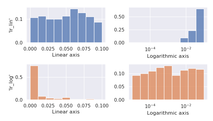
Hyperparameters often span over multiple orders of magnitude. For instance, the optimal learning rate of a neural network
could be in the range from 0.00001 to 0.1.
Drawing uniform samples from this range favors larger values, as the center of the interval is approximately 0.05, which means that half of all generated samples will be larger than 0.05 on average.
For such parameters, logarithmic sampling, enabled via the log argument, is a better option
search = pyhopper.Search(
    {
        "dropout": pyhopper.float(0, 0.5),
        "lr_lin": pyhopper.float(1e-5, 1e-1),           # linear
        "lr_log": pyhopper.float(1e-5, 1e-1, log=True), # logarithmic
    }
)
> {"dropout": 0.11816788326, "lr_lin": 0.05527447103, "lr_log": 0.00123320712}
> {"dropout": 0.03368100192, "lr_lin": 0.04697054821, "lr_log": 0.00001454088}
> {"dropout": 0.19095931974, "lr_lin": 0.00770115557, "lr_log": 0.02469411646}
> {"dropout": 0.13041185714, "lr_lin": 0.05653078541, "lr_log": 0.00185817307}
> {"dropout": 0.29153194475, "lr_lin": 0.08468031050, "lr_log": 0.04448428726}
Looking at the histogram of both parameters’ samples illustrates this effect better:
Keeping all digits of a float parameter looks ugly and increases the chance of overfitting.
To limit the precision, we can use the precision argument.
precision defines the number of digits after the comma in the default linear sampling mode, whereas the number of significant digits in the logarithmic mode.
search = pyhopper.Search(
    {
        "dropout": pyhopper.float(0, 0.5, precision=2),          # 2 digits after the comma
        "lr": pyhopper.float(1e-5, 1e-1, log=True, precision=1), # 1 significant digit
    }
)
> {'dropout': 0.04, 'lr': 0.0001}
> {'dropout': 0.11, 'lr': 0.02}
> {'dropout': 0.37, 'lr': 0.008}
> {'dropout': 0.13, 'lr': 0.0001}
> {'dropout': 0.20, 'lr': 0.0009}
Note
The precision and log arguments can also be set via the fmt (format string) argument. For instance, fmt=”0.2f”` is short for log=False, precision=2, and fmt=”0.1g” is short for log=True, precision=1.
search = pyhopper.Search(
    {
        "dropout": pyhopper.float(0, 0.5, "0.2f"), # 2 digits after the comma (linear)
        "lr": pyhopper.float(1e-5, 1e-1, "0.1g"), # 1 significant digit (logarithmic)
    }
)
pyhopper.choice() requires a list of possible values for this hyperparameter.
Similar to before, we can provide an initial guess.
In case the values in the list are provided in a structured order, setting the is_ordinal argument indicates pyhopper to preserve this order when sampling.
For instance in
search = pyhopper.Search(
    {
        "opt": pyhopper.choice(["adam", "rmsprop", "sgd"]),
        "dropout": pyhopper.choice([0, 0.1, 0.2, 0.3], is_ordinal=True),
    }
)
the parameter "opt" has no ordering but "dropout" has, making pyhopper sample items adjacent to the current best value.
{'opt': 'adam', 'dropout': 0.3}
{'opt': 'adam', 'dropout': 0.2}
{'opt': 'sgd', 'dropout': 0.3}
Running PyHopper#
Once we have defined the search space, we can schedule the search using the pyhopper.Search.run() method.
The method requires three argument: The objective function, the direction of the search (minimize or maximize), and the runtime of the search.
For specifying the runtime, we can provide a string that is parsed by pyhopper.parse_runtime() or simply an integer/float with the runtime in seconds.
runtime = 30               # 30 seconds
runtime = "2h 10min"       # 2 hours and 10 minutes
runtime = "3d 7h 30m 10s"  # 3 days, 7 hours, 30 minute and 10 seconds
To utilize multi CPU/GPU hardware, we can run multiple evaluations of parameter candidates in parallel with the n_jobs argument.
For instance,
import pyhopper
import time

def of(param):
    time.sleep(1)      # some slow code
    return param["x"]

search = pyhopper.Search({"x": pyhopper.float(0, 1)})

start = time.time()
search.run(of, steps=20, quiet=True)
print(f"n_jobs=1 took {time.time()-start:0.2f} seconds")

start = time.time()
search.run(of, steps=20, quiet=True, n_jobs=4)
print(f"n_jobs=4 took {time.time()-start:0.2f} seconds")
> n_jobs=1 took 20.19 seconds
> n_jobs=4 took 5.08 seconds
Setting the argument to n_jobs="per-gpu" will spawn exactly one worker process for each GPU attached to the machine.
Moreover, PyHopper will take care of setting the CUDA_VISIBLE_DEVICES environment variable for each of the worker processes to its private GPU, so each worker sees only a single GPU.
Consequently, we can write standard PyTorch and TensorFlow code in the objective function without having to worry about two processes accessing the same device.
TL;DR: useful values for n_jobs are:
n_jobs = 1            # No parallel workers
n_jobs = 4            # 4 parallel workers
n_jobs = "per-gpu"    # A worker for each GPU device
n_jobs = "2x per-gpu" # 2 workers for each GPU device
n_jobs = -1           # A worker for each CPU core
A putting things together#
Putting everything together, a typical hyperparameter tuning code may look something like this
import pyhopper

def my_objective(param: dict) -> float:
    # Add code here
    return val_acc

search = pyhopper.Search(
    {
        "epochs": 20,
        "num_layers": pyhopper.int(1, 8, init=4),
        "batch_size": pyhopper.int(32, 512, multiple_of=32),
        "dropout": pyhopper.float(0, 0.5, precision=1),
        "lr": pyhopper.float(1e-5, 1e-2, log=True, precision=1),
        "opt": pyhopper.choice(["adam", "rmsprop", "sgd"], init="adam"),
        "weight_decay": pyhopper.choice([0, 1e-5, 1e-4, 1e-3], is_ordinal=True),
    }
)
search.run(my_objective, "max", "4h", n_jobs="per-gpu")
Further topics#
The following topics give us some peak into the capabilities of Pyhopper.
Checkpointing#
We can automatically save the search progress in a checkpoint file, so if the process is interrupted (for instance by the shutdown of a pre-emptive cloud instance) we can resume the process where it left off.
search = pyhopper.Search( ... )

search.run(
    objective, "minimize", "12h",
    checkpoint_path = "my_checkpoint.ckpt"

search.save("run_completed.ckpt")
# search.load("run_completed.ckpt")
If the file checkpoint_path already exists, Pyhopper will try to load it and resume the remaining search.
At the end of the search, the file will not be deleted and we can use it extend the search, for instance, running it for another day if we are not satisfied with the results.
For further details see Checkpointing
Dealing with a noisy objective#
Training a neural network is an inherently stochastic process. Randomness from the weight initialization has a strong influence on the final accuracy.
In the context of a hyperparameter search, it may happen that a non-optimal parameter candidate achieves a high accuracy by simply having luck with the initial weights used for its evaluation.
To tell spurious and genuine high accuracy apart, we have to evaluate each parameter candidate several times and use the average accuracy as our objective metric.
For exactly this reason, PyHopper provides the pyhopper.wrap_n_times() function that wraps an arbitrary function into its mean over n evaluations.
def noisy_objective(param):
    print(param["name"])
    return 0

search = pyhopper.Search({"name": pyhopper.choice(["adam","eve"])})

search.run(
    pyhopper.wrap_n_times(noisy_objective,3),
    "minimize",
    "3s"
)
> adam
> adam
> adam
> eve
> eve
> eve
Note
To reduce the computational cost of evaluating each candidate multiple times, PyHopper allows cancelling candidates if their first evaluation shows that they have only a small chance of becoming the best hyperparameters. See Pruners for more details.
Pruners#
When wrapping an objective function with `pyhopper.wrap_n_times(noisy_objective,3)`, we can potentially save a lot of compute if we discontinue an unpromising candidate after the evaluation.
For instance, if our current best parameters evaluate to an accuracy of 95%, and a sampled candidate evaluates to 70% in the first evaluation, it does not make sense to evaluate the candidate two more times.
Instead, we can prune the candidate.
search = pyhopper.Search(...)

search.run(
    pyhopper.wrap_n_times(noisy_objective,3),
    "maximize",
    steps=50,
    pruner = pyhopper.pruners.QuantilePruner(0.8) # discontinue candidates if they are in the bottom 80%
)
> Search is scheduled for 50 steps
> Current best 0.0596: 100%|█████████████████████████| 50/50 [00:00<00:00, 101.45steps/s]
> ======================= Summary ======================
> Mode              : Best f : Steps : Pruned    : Time
> -----------       : ---    : ---   : ---       : ---
> Initial solution  : -4.09  : 1     : 0         : 9 ms
> Random seeding    : 0.0596 : 6     : 43        : 60 ms
> -----------       : ---    : ---   : ---       : ---
> Total             : 0.0596 : 7     : 43        : 69 ms
> ======================================================
For further details, see Pruners.
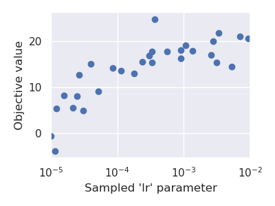
Accessing the search history#
Pyhopper keeps track of all evaluated parameter candidates and corresponding objective value in the Search.history property.
We can, for instance, use this history to examine or visualize the search space.
search = pyhopper.Search(
    {
        "lr": pyhopper.float(1e-5,1e-2,log=True),
    }
)
search.run(...)

fig, ax = plt.subplots(figsize=(4, 3))
b = ax.scatter(
    x=search.history["lr"],
    y=search.history.fs,
)
ax.set_xlabel("Sampled 'lr' parameter")
ax.set_ylabel("Objective value")
ax.set_xscale("log")
plt.show(fig)
For further details see See Search history.